
Binary Classification - Cats and Dogs
In this tutorial, we will walk through several iterations of a classification model that distinguishes between cats and dogs.
Setup
To set up, let us import a few useful libraries to help us plot some examples and run the models.
import os
from tensorflow.keras import utils
import tensorflow as tf
from tensorflow.keras import layers
import matplotlib.pyplot as plt
Now, we download the open source data using the utils library in tensorflow.keras. This dataset has already been segmented into training and validation sets, so we can access these datasets by their specific filepaths. We can construct testing dataset from the validation dataset by picking out every 5th image using the .skip() function.
# location of data
_URL = 'https://storage.googleapis.com/mledu-datasets/cats_and_dogs_filtered.zip'

# download the data and extract it
path_to_zip = utils.get_file('cats_and_dogs.zip', origin=_URL, extract=True)

# construct paths
PATH = os.path.join(os.path.dirname(path_to_zip), 'cats_and_dogs_filtered')

train_dir = os.path.join(PATH, 'train')
validation_dir = os.path.join(PATH, 'validation')

# parameters for datasets
BATCH_SIZE = 32
IMG_SIZE = (160, 160)

# construct train and validation datasets
train_dataset = utils.image_dataset_from_directory(train_dir, shuffle=True, batch_size=BATCH_SIZE,image_size=IMG_SIZE)

validation_dataset = utils.image_dataset_from_directory(validation_dir,
                                                        shuffle=True,
                                                        batch_size=BATCH_SIZE,
                                                        image_size=IMG_SIZE)

# construct the test dataset by taking every 5th observation out of the validation dataset
val_batches = tf.data.experimental.cardinality(validation_dataset)
test_dataset = validation_dataset.take(val_batches // 5)
validation_dataset = validation_dataset.skip(val_batches // 5)
Found 2000 files belonging to 2 classes.
Found 1000 files belonging to 2 classes.
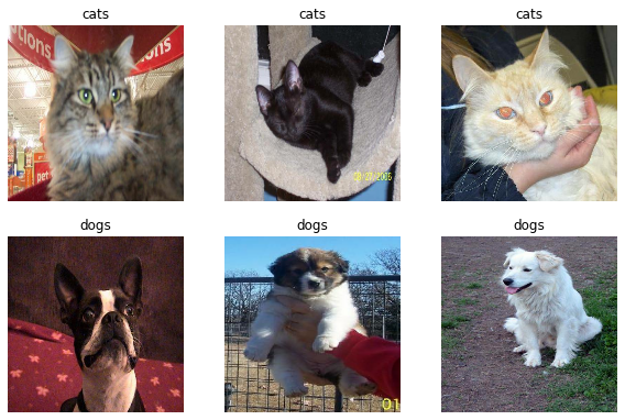
We can view a sample of this dataset using pyplot:
def plot_classes(dataset):
  class_names = dataset.class_names
  plt.figure(figsize=(10, 10))
  for pairs in dataset.take(1):
    # retrieve images of cats
    cats = [pairs[0][i].numpy().astype("uint8") for i in range(len(pairs[1])) if pairs[1][i] == 0][:3]

    # append images of dogs to add to second row
    cats_and_dogs = cats + [pairs[0][i].numpy().astype("uint8") for i in range(len(pairs[1])) if pairs[1][i] == 1][:3]
    for i in range(6):
      ax = plt.subplot(3, 3, i + 1)
      plt.imshow(cats_and_dogs[i])
      plt.title('cats' if i < 3 else 'dogs')
      plt.axis("off")

plot_classes(train_dataset)
The next block allows for rapid reading of data.
AUTOTUNE = tf.data.AUTOTUNE

train_dataset = train_dataset.prefetch(buffer_size=AUTOTUNE)
validation_dataset = validation_dataset.prefetch(buffer_size=AUTOTUNE)
test_dataset = test_dataset.prefetch(buffer_size=AUTOTUNE)
Model
To begin, we evaluate the baseline accuracy of our model. We calculate the probability of selecting a dog image given a uniformly random pick from the training dataset.
labels_iterator= train_dataset.unbatch().map(lambda image, label: label).as_numpy_iterator()
length, numdogs = 0,0

# iterate over labels set - add 1 for dog class
for i in labels_iterator:
  length += 1
  numdogs += i

numdogs / float(length)
0.5
Thus, our model should be viable if the validation and testing accuracies surpass 50%.
Next, we define the loss function that allows the model to update weights:
loss_fn = tf.keras.losses.SparseCategoricalCrossentropy(from_logits=True) # this is our q_i
First Iteration
In this iteration of the model, we include several three convolution layers, two max pooling layers, one flatten layer, and two dense layers at the end. The relu function is the most efficient choice for activation.
model1 = tf.keras.models.Sequential([
      layers.Conv2D(32, (3, 3), activation='relu', input_shape=(160, 160, 3)),
      layers.MaxPooling2D((2, 2)),
      layers.Conv2D(32, (3, 3), activation='relu'),
      layers.MaxPooling2D((2, 2)),
      layers.Conv2D(64, (3, 3), activation='relu'),
      layers.Flatten(), # flattens into 1D vector

      layers.Dense(64, activation='relu'),
      layers.Dense(2) # number of classes in your dataset
])
Now, we compile and train our first model:
model1.compile(optimizer='adam',
             loss = loss_fn,
              metrics = ['accuracy'])

history = model1.fit(train_dataset,
                     epochs=20,
                     validation_data=validation_dataset)
Epoch 1/20
63/63 [==============================] - 72s 1s/step - loss: 14.1985 - accuracy: 0.5460 - val_loss: 0.6877 - val_accuracy: 0.5557
Epoch 2/20
63/63 [==============================] - 68s 1s/step - loss: 0.6074 - accuracy: 0.6785 - val_loss: 0.7089 - val_accuracy: 0.5656
Epoch 3/20
63/63 [==============================] - 67s 1s/step - loss: 0.4532 - accuracy: 0.7795 - val_loss: 0.7696 - val_accuracy: 0.5569
Epoch 4/20
63/63 [==============================] - 68s 1s/step - loss: 0.3119 - accuracy: 0.8700 - val_loss: 1.1004 - val_accuracy: 0.5693
Epoch 5/20
63/63 [==============================] - 68s 1s/step - loss: 0.1628 - accuracy: 0.9445 - val_loss: 1.5570 - val_accuracy: 0.5730
Epoch 6/20
63/63 [==============================] - 67s 1s/step - loss: 0.0824 - accuracy: 0.9735 - val_loss: 1.5398 - val_accuracy: 0.5582
Epoch 7/20
63/63 [==============================] - 68s 1s/step - loss: 0.0565 - accuracy: 0.9880 - val_loss: 1.7233 - val_accuracy: 0.6052
Epoch 8/20
63/63 [==============================] - 67s 1s/step - loss: 0.0145 - accuracy: 0.9970 - val_loss: 1.8505 - val_accuracy: 0.5879
Epoch 9/20
63/63 [==============================] - 67s 1s/step - loss: 0.0093 - accuracy: 0.9995 - val_loss: 2.3999 - val_accuracy: 0.6064
Epoch 10/20
63/63 [==============================] - 68s 1s/step - loss: 0.0168 - accuracy: 0.9955 - val_loss: 1.8899 - val_accuracy: 0.5507
Epoch 11/20
63/63 [==============================] - 68s 1s/step - loss: 0.0302 - accuracy: 0.9945 - val_loss: 2.1095 - val_accuracy: 0.6151
Epoch 12/20
63/63 [==============================] - 67s 1s/step - loss: 0.0049 - accuracy: 0.9990 - val_loss: 2.4323 - val_accuracy: 0.6002
Epoch 13/20
63/63 [==============================] - 67s 1s/step - loss: 0.0088 - accuracy: 0.9985 - val_loss: 2.2477 - val_accuracy: 0.5978
Epoch 14/20
63/63 [==============================] - 67s 1s/step - loss: 0.0076 - accuracy: 0.9985 - val_loss: 2.3757 - val_accuracy: 0.6027
Epoch 15/20
63/63 [==============================] - 67s 1s/step - loss: 0.0513 - accuracy: 0.9840 - val_loss: 2.2290 - val_accuracy: 0.5545
Epoch 16/20
63/63 [==============================] - 67s 1s/step - loss: 0.1108 - accuracy: 0.9770 - val_loss: 2.1335 - val_accuracy: 0.5916
Epoch 17/20
63/63 [==============================] - 67s 1s/step - loss: 0.0391 - accuracy: 0.9910 - val_loss: 2.1000 - val_accuracy: 0.5965
Epoch 18/20
63/63 [==============================] - 67s 1s/step - loss: 0.0295 - accuracy: 0.9935 - val_loss: 1.9495 - val_accuracy: 0.5879
Epoch 19/20
63/63 [==============================] - 67s 1s/step - loss: 0.0218 - accuracy: 0.9940 - val_loss: 2.0806 - val_accuracy: 0.5953
Epoch 20/20
63/63 [==============================] - 67s 1s/step - loss: 0.0023 - accuracy: 0.9995 - val_loss: 2.2627 - val_accuracy: 0.6089
This model was the most straightforward in terms of achieving the required accuracy. However, a few other parameters were tested to try and improve the validation accuracy. For example, we tested the model with 64 filters for the first two 2D convolution layers. However, setting to 32 filters yielded a more accurate model. Our validation accuracy stabilizes between 55% and 60%. However, the model is severely overfitted to the training data, which explains the discrepancy between the training and validation accuracies. Thus, while this model is better than the baseline, we can do better. Let’s see how we can improve this metric by preprocessing and transforming the data.
Model 2
To begin our second model, we construct a data augmentation layer that rotates and flips the data. This ensures that our model learns to account for image transformations that do not change the features of a dog or cat.
First, let us look at two examples of the augmentation being applied to our training set:
data_augmentation = tf.keras.Sequential([
  tf.keras.layers.RandomFlip('horizontal'),
  tf.keras.layers.RandomRotation(0.2), # randomly rotate by at most a factor of 0.2*pi
])

for image, _ in train_dataset.take(1):
  plt.figure(figsize=(10, 10))

  # create four images: two originals and two augmentations
  first_images = [tf.expand_dims(im, 0) for im in [image[0], image[1]]]
  ims = [(im, data_augmentation(im)) for im in first_images]

  #unpacks the original-augmented pairs for plotting
  images_unpacked = [a for tup in ims for a in tup]
  for i in range(4):
    ax = plt.subplot(2, 2, i + 1)
    plt.imshow(images_unpacked[i][0] / 255)
    plt.axis('off')
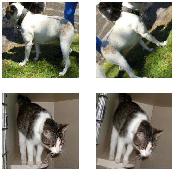
Next, we will train a sequential model that uses the augmentation layer defined in the previous section. The addition of the augmentation layer negatively affected our validation accuracy. Simply adding the augmentation layer to the setup of model 1 was not sufficient for meeting the higher benchmark required of this part. Using the sigmoid activation function also did not yield any marked improvements. It seemed that condensing the number of operations helped improve this model’s accuracy and overfitting problem. Thus, we retained only one convolution layer, the flattening layer, and the dense layer (this last one is still needed to adjust for the number of classes).
model2 = tf.keras.models.Sequential([
      data_augmentation,
      layers.Conv2D(64, (3, 3), activation='relu', input_shape=(160, 160, 3)),
      layers.Flatten(),
      layers.Dense(2)
])

model2.compile(optimizer='adam',
             loss = loss_fn,
              metrics = ['accuracy'])

history2 = model2.fit(train_dataset,
                     epochs=20,
                     validation_data=validation_dataset)
Epoch 1/20
63/63 [==============================] - 49s 756ms/step - loss: 1013.4577 - accuracy: 0.5300 - val_loss: 8.7492 - val_accuracy: 0.5730
Epoch 2/20
63/63 [==============================] - 53s 845ms/step - loss: 7.1085 - accuracy: 0.5550 - val_loss: 6.4506 - val_accuracy: 0.5458
Epoch 3/20
63/63 [==============================] - 59s 933ms/step - loss: 4.1212 - accuracy: 0.5515 - val_loss: 4.7688 - val_accuracy: 0.5631
Epoch 4/20
63/63 [==============================] - 47s 743ms/step - loss: 2.5457 - accuracy: 0.5845 - val_loss: 4.4762 - val_accuracy: 0.5520
Epoch 5/20
63/63 [==============================] - 47s 746ms/step - loss: 2.9172 - accuracy: 0.5840 - val_loss: 5.6308 - val_accuracy: 0.5384
Epoch 6/20
63/63 [==============================] - 53s 845ms/step - loss: 2.6828 - accuracy: 0.5965 - val_loss: 4.6006 - val_accuracy: 0.5309
Epoch 7/20
63/63 [==============================] - 48s 749ms/step - loss: 2.1590 - accuracy: 0.6055 - val_loss: 3.6583 - val_accuracy: 0.5198
Epoch 8/20
63/63 [==============================] - 46s 734ms/step - loss: 2.5018 - accuracy: 0.5955 - val_loss: 2.8134 - val_accuracy: 0.5483
Epoch 9/20
63/63 [==============================] - 47s 740ms/step - loss: 1.7107 - accuracy: 0.5620 - val_loss: 2.5899 - val_accuracy: 0.5297
Epoch 10/20
63/63 [==============================] - 46s 732ms/step - loss: 1.4004 - accuracy: 0.6040 - val_loss: 2.4268 - val_accuracy: 0.5470
Epoch 11/20
63/63 [==============================] - 47s 735ms/step - loss: 1.4149 - accuracy: 0.5985 - val_loss: 2.1249 - val_accuracy: 0.5582
Epoch 12/20
63/63 [==============================] - 46s 727ms/step - loss: 1.1450 - accuracy: 0.6065 - val_loss: 2.0807 - val_accuracy: 0.5545
Epoch 13/20
63/63 [==============================] - 47s 735ms/step - loss: 1.0127 - accuracy: 0.5990 - val_loss: 2.0231 - val_accuracy: 0.5557
Epoch 14/20
63/63 [==============================] - 46s 730ms/step - loss: 1.0314 - accuracy: 0.5980 - val_loss: 1.8393 - val_accuracy: 0.5545
Epoch 15/20
63/63 [==============================] - 46s 731ms/step - loss: 1.0250 - accuracy: 0.6185 - val_loss: 1.8457 - val_accuracy: 0.5495
Epoch 16/20
63/63 [==============================] - 46s 727ms/step - loss: 0.9460 - accuracy: 0.6195 - val_loss: 1.7879 - val_accuracy: 0.5582
Epoch 17/20
63/63 [==============================] - 46s 728ms/step - loss: 0.8990 - accuracy: 0.6175 - val_loss: 1.7391 - val_accuracy: 0.5520
Epoch 18/20
63/63 [==============================] - 46s 729ms/step - loss: 0.9147 - accuracy: 0.6145 - val_loss: 1.7254 - val_accuracy: 0.5545
Epoch 19/20
63/63 [==============================] - 46s 729ms/step - loss: 0.8481 - accuracy: 0.6145 - val_loss: 1.6334 - val_accuracy: 0.5582
Epoch 20/20
63/63 [==============================] - 46s 727ms/step - loss: 0.8748 - accuracy: 0.5955 - val_loss: 1.4964 - val_accuracy: 0.5532
This model consistently scores 55% validation accuracy. This model is actually less accurate than the previous one but does address the overfitting problem since the training and validation accuracies are more comparable. Thus, we can strategically add more layers around the data augmentation layer to create more accurate models that are not in danger of overfitting.
Model 3
In our third model, we will add a preprocessor before the data augmentation layer. We can achieve this normalizing the color scale to values between 0 and 1 so that the model spends fewer iterations adjusting the weights to the original color scale (0 to 255). This should improve our validation accuracy.
# Add preprocessor
i = tf.keras.Input(shape=(160, 160, 3))
x = tf.keras.applications.mobilenet_v2.preprocess_input(i)
preprocessor = tf.keras.Model(inputs = [i], outputs = [x])

model3 = tf.keras.models.Sequential([
      data_augmentation,
      preprocessor,
      layers.Conv2D(32, (3, 3), activation='relu', input_shape=(160, 160, 3)),
      layers.MaxPooling2D((2, 2)),
      layers.Conv2D(32, (3, 3), activation='relu'),
      layers.MaxPooling2D((2, 2)),
      layers.Conv2D(64, (3, 3), activation='relu'),
      layers.Flatten(),
      layers.Dense(64, activation='relu'),
      layers.Dense(2)
])

model3.compile(optimizer='adam', # fancier version of SGD
             loss = loss_fn,
              metrics = ['accuracy'])  # you can add callbacks

history3 = model3.fit(train_dataset,
                     epochs=20,
                     validation_data=validation_dataset)
Epoch 1/20
63/63 [==============================] - 75s 1s/step - loss: 0.7309 - accuracy: 0.5535 - val_loss: 0.6714 - val_accuracy: 0.5916
Epoch 2/20
63/63 [==============================] - 73s 1s/step - loss: 0.6566 - accuracy: 0.5960 - val_loss: 0.6355 - val_accuracy: 0.6188
Epoch 3/20
63/63 [==============================] - 73s 1s/step - loss: 0.6326 - accuracy: 0.6405 - val_loss: 0.6631 - val_accuracy: 0.6188
Epoch 4/20
63/63 [==============================] - 73s 1s/step - loss: 0.6108 - accuracy: 0.6590 - val_loss: 0.6339 - val_accuracy: 0.6436
Epoch 5/20
63/63 [==============================] - 73s 1s/step - loss: 0.5882 - accuracy: 0.6800 - val_loss: 0.6185 - val_accuracy: 0.6448
Epoch 6/20
63/63 [==============================] - 72s 1s/step - loss: 0.5965 - accuracy: 0.6850 - val_loss: 0.6313 - val_accuracy: 0.6535
Epoch 7/20
63/63 [==============================] - 72s 1s/step - loss: 0.5758 - accuracy: 0.6890 - val_loss: 0.7225 - val_accuracy: 0.6225
Epoch 8/20
63/63 [==============================] - 72s 1s/step - loss: 0.5817 - accuracy: 0.6800 - val_loss: 0.6319 - val_accuracy: 0.6423
Epoch 9/20
63/63 [==============================] - 73s 1s/step - loss: 0.5727 - accuracy: 0.6925 - val_loss: 0.5815 - val_accuracy: 0.7005
Epoch 10/20
63/63 [==============================] - 72s 1s/step - loss: 0.5599 - accuracy: 0.7090 - val_loss: 0.5889 - val_accuracy: 0.7141
Epoch 11/20
63/63 [==============================] - 72s 1s/step - loss: 0.5605 - accuracy: 0.7000 - val_loss: 0.6220 - val_accuracy: 0.6881
Epoch 12/20
63/63 [==============================] - 72s 1s/step - loss: 0.5388 - accuracy: 0.7265 - val_loss: 0.5763 - val_accuracy: 0.7166
Epoch 13/20
63/63 [==============================] - 72s 1s/step - loss: 0.5373 - accuracy: 0.7310 - val_loss: 0.5906 - val_accuracy: 0.7079
Epoch 14/20
63/63 [==============================] - 73s 1s/step - loss: 0.5367 - accuracy: 0.7250 - val_loss: 0.5672 - val_accuracy: 0.7166
Epoch 15/20
63/63 [==============================] - 72s 1s/step - loss: 0.5185 - accuracy: 0.7325 - val_loss: 0.6360 - val_accuracy: 0.6955
Epoch 16/20
63/63 [==============================] - 73s 1s/step - loss: 0.5195 - accuracy: 0.7370 - val_loss: 0.5679 - val_accuracy: 0.7339
Epoch 17/20
63/63 [==============================] - 73s 1s/step - loss: 0.5296 - accuracy: 0.7320 - val_loss: 0.5386 - val_accuracy: 0.7277
Epoch 18/20
63/63 [==============================] - 73s 1s/step - loss: 0.5066 - accuracy: 0.7460 - val_loss: 0.5685 - val_accuracy: 0.7240
Epoch 19/20
63/63 [==============================] - 72s 1s/step - loss: 0.5056 - accuracy: 0.7435 - val_loss: 0.5982 - val_accuracy: 0.7191
Epoch 20/20
63/63 [==============================] - 72s 1s/step - loss: 0.5128 - accuracy: 0.7525 - val_loss: 0.5816 - val_accuracy: 0.7215
We reuse the same setup as model 1 in this segment, and the addition of the preprocessing makes up for the lower validation accuracy caused by the addition of the data augmentation layer. This model consistently achieved 70% to 73% validation accuracy. This is a significant improvement compared to model 1. Overfitting does not seem to be a concern since the training and validation accuracies are fairly similar.
Model 4
Our final iteration of the model introduces a base model on which we add our own layers. This base model will have already learned over a similar set of data, so our model will learn weights for this specific problem more quickly. For this model, we find that a very minimal number of layers still meets the required specs. In addition to the preprocessor, data augmentation, and base model layers, we have a flattening layer and two dense layers, the last of which performs the actual classification. While we anticipated having to add a global max pooling layer as well, there seems to have been no need for it, as we see below.
IMG_SHAPE = IMG_SIZE + (3,)

# access base model as is
base_model = tf.keras.applications.MobileNetV2(input_shape=IMG_SHAPE,
                                               include_top=False,
                                               weights='imagenet')
base_model.trainable = False

i = tf.keras.Input(shape=IMG_SHAPE)
x = base_model(i, training = False)
base_model_layer = tf.keras.Model(inputs = [i], outputs = [x])

model4 = tf.keras.models.Sequential([
      preprocessor,
      layers.RandomFlip(), # flips horizontal or vertical
      tf.keras.layers.RandomRotation(factor=(-2, 2)),
      base_model_layer,
      layers.Flatten(),
      layers.Dense(64, activation='relu'),
      layers.Dense(2)
])

model4.compile(optimizer='adam',
             loss = loss_fn,
              metrics = ['accuracy'])

history = model4.fit(train_dataset,
                     epochs=20,
                     validation_data=validation_dataset)
Epoch 1/20
63/63 [==============================] - 51s 762ms/step - loss: 1.0066 - accuracy: 0.8265 - val_loss: 0.0829 - val_accuracy: 0.9752
Epoch 2/20
63/63 [==============================] - 48s 757ms/step - loss: 0.2623 - accuracy: 0.8995 - val_loss: 0.0747 - val_accuracy: 0.9740
Epoch 3/20
63/63 [==============================] - 48s 756ms/step - loss: 0.1969 - accuracy: 0.9185 - val_loss: 0.0698 - val_accuracy: 0.9765
Epoch 4/20
63/63 [==============================] - 48s 756ms/step - loss: 0.1651 - accuracy: 0.9365 - val_loss: 0.0716 - val_accuracy: 0.9752
Epoch 5/20
63/63 [==============================] - 48s 757ms/step - loss: 0.1516 - accuracy: 0.9340 - val_loss: 0.0619 - val_accuracy: 0.9777
Epoch 6/20
63/63 [==============================] - 48s 753ms/step - loss: 0.1481 - accuracy: 0.9475 - val_loss: 0.0760 - val_accuracy: 0.9752
Epoch 7/20
63/63 [==============================] - 48s 754ms/step - loss: 0.1403 - accuracy: 0.9475 - val_loss: 0.0993 - val_accuracy: 0.9629
Epoch 8/20
63/63 [==============================] - 48s 753ms/step - loss: 0.1419 - accuracy: 0.9465 - val_loss: 0.0757 - val_accuracy: 0.9752
Epoch 9/20
63/63 [==============================] - 48s 754ms/step - loss: 0.1333 - accuracy: 0.9485 - val_loss: 0.0699 - val_accuracy: 0.9765
Epoch 10/20
63/63 [==============================] - 47s 752ms/step - loss: 0.1230 - accuracy: 0.9495 - val_loss: 0.0853 - val_accuracy: 0.9678
Epoch 11/20
63/63 [==============================] - 47s 752ms/step - loss: 0.1142 - accuracy: 0.9540 - val_loss: 0.0792 - val_accuracy: 0.9691
Epoch 12/20
63/63 [==============================] - 48s 755ms/step - loss: 0.1135 - accuracy: 0.9535 - val_loss: 0.0810 - val_accuracy: 0.9703
Epoch 13/20
63/63 [==============================] - 48s 761ms/step - loss: 0.1090 - accuracy: 0.9580 - val_loss: 0.0723 - val_accuracy: 0.9740
Epoch 14/20
63/63 [==============================] - 47s 752ms/step - loss: 0.1095 - accuracy: 0.9510 - val_loss: 0.0697 - val_accuracy: 0.9802
Epoch 15/20
63/63 [==============================] - 48s 768ms/step - loss: 0.1194 - accuracy: 0.9505 - val_loss: 0.0993 - val_accuracy: 0.9604
Epoch 16/20
63/63 [==============================] - 48s 765ms/step - loss: 0.0979 - accuracy: 0.9590 - val_loss: 0.1068 - val_accuracy: 0.9567
Epoch 17/20
63/63 [==============================] - 49s 771ms/step - loss: 0.0896 - accuracy: 0.9665 - val_loss: 0.0927 - val_accuracy: 0.9691
Epoch 18/20
63/63 [==============================] - 48s 768ms/step - loss: 0.0838 - accuracy: 0.9655 - val_loss: 0.0939 - val_accuracy: 0.9715
Epoch 19/20
63/63 [==============================] - 48s 760ms/step - loss: 0.1001 - accuracy: 0.9575 - val_loss: 0.0919 - val_accuracy: 0.9703
Epoch 20/20
63/63 [==============================] - 48s 761ms/step - loss: 0.0999 - accuracy: 0.9565 - val_loss: 0.0931 - val_accuracy: 0.9666
Our validation accuracy stabilizes between 95% and 97%, which is a highly significant improvement over all the previous models. We do not observe a problem with overfitting because the validation accuracy proves to be consistently on the same level as the testing accuracy.
Testing
Finally, we look to evaluate model 4 against the testing set using the evaluate() function.
model4.evaluate(test_dataset)
6/6 [==============================] - 3s 491ms/step - loss: 0.0503 - accuracy: 0.9844


[0.050344910472631454, 0.984375]
As we can see, the final iteration of the model is a competent classifier.